Continuous profiling

See where a service spends CPU or allocates memory, down to the function. Oriel ingests OTLP profiles, the development-stage fourth signal, alongside traces, logs, and metrics. Each profile arrives heavily normalized: a sample points at a stack in a shared dictionary, where a stack indexes locations and a location indexes functions. Oriel resolves that dictionary once at ingest and stores one row per distinct call path, so a flamegraph is a single sum(value) grouped by stack.

Profiles ride the same pipeline as the other signals: the ingest token, project and environment resolution, the timestamp window, and per-project retention all apply unchanged.

Send profiles

Profiles use the OTLP profiles service over gRPC on :4317 and HTTP on :4318 at /v1/profiles. Create an ingest token under workspace settings and include the profiles signal; a token created without an explicit signal restriction carries it by default.

Any OTLP profiles producer works. The reference host-level producer is opentelemetry-ebpf-profiler, a whole-system eBPF profiler that samples every process at about 1% CPU overhead with no application changes or redeploys. Configure its OTLP collection endpoint to the ingest gRPC address and pass the ingest token as an Authorization: Bearer header; the project’s README lists the current flags for the endpoint, TLS, and headers.

Language SDKs that emit OTLP profiles send to the same endpoint. A sample that carries a span link is stored with its trace and span id, which is what makes the trace-to-profile jump below work.

Retention

Profile volume is high, so profiles keep their own per-project retention, retention_profiles_days, defaulting to 7 days. Set it per project the same way as the other signals:

curl -X PATCH https://oriel.example.com/api/v1/workspaces/demo/projects/$PJ \
  -H "Authorization: Bearer $API_TOKEN" \
  -d '{"retention_profiles_days": 3}'

A row’s retention is stamped at ingest, so a change applies to profiles received after it.

Read profiles

The Profiles screen renders a flamegraph for the service and time range in the top bar. When more than one profile type is present (cpu, allocations, and so on), a picker switches between them; the value axis follows the type’s unit, so cpu shows as time and allocations as bytes. Click a frame to zoom into its subtree and Reset zoom to return. The hottest paths sort left-first.

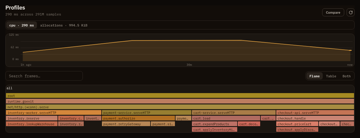
Use Compare to select two windows and render a diff flamegraph for the same profile type and filter. Each frame carries both window values, so regressions and improvements stay attached to their call path instead of becoming separate tables. Compare mode is for range-to-range analysis; trace-pinned profile views show the sampled trace window instead.

Use the sandwich view when a single function needs context. Select a function from the profile table or flamegraph to see its caller and callee neighborhood in the active range. The same profile type, scope, filter, and optional trace_id apply.

Profiles are also a first-class OQL source, so they chart and aggregate like any other signal. Stack counts per service:

profiles | where profile_type == "cpu" | stats sum(value) as cpu by service | top 10 by cpu

Resource attributes live in the one attribute map, reachable by their bare name (profiles | where host_name == "web-1"). Profiles do not carry the resource. prefix or numeric attribute maps that spans and logs do.

Link a profile to a trace

A sample whose OTLP link names a trace is stored with that trace and span id. The flamegraph endpoint accepts a trace_id, so a trace’s detail page links straight to the profile sampled while that trace ran: open a trace and follow view profile. The Profiles screen then shows only the stacks sampled under that trace, with a control to clear the filter. This reuses the same trace-id linking that exemplars use to tie a metric spike back to an example trace.